Basics of Machine Learning, Algorithms and Applications
What is Machine Learning (ML)?
“Data is abundant and cheap but knowledge is scarce and expensive.”
Have a look at the exciting ~ 4mins video below.
It gives an idea of how machine learning is making computers, and many of the things like maps, search, recommending videos, translations, etc. better.
機器學習, 或者叫人工智能
其實研究機器學習也就是研究人類如何學習,或者研究智能是怎麼形成的,或者叫智能形成的模式,方法
At the end of this article, you will be familiar with the basic concepts of machine learning, types of machine learning, its applications, and a lot more.
Let us begin by addressing the elephant in the room.
The search engines (Google, Bing, Duckduckgo) have become the new knowledge discovery platforms.
They have answers (probably accurate) to almost every silly question you can think of ? But, how did it become so intelligent? Think about it!
In the meanwhile, let us first look at a few definitions of machine learning.
The term “machine learning” was coined by Arthur Samuel in 1959. According to him,
"Machine learning is the subfield of computer science that gives computers the ability to learn without being explicitly programmed."
Tom M. Mitchell provided a more formal definition, which says,
"A computer program is said to learn from experience E with respect to some class of tasks T and performance measure P if its performance at tasks in T, as measured by P, improves with experience E."
What are the different types of ML algorithms?
For better understanding, ML algorithms and techniques have been divided into 3 major categories.
1. Supervised Learning
It is one of the most commonly used types of machine learning algorithms.
In these types of ML algorithms, we have input and output variables and the algorithm generates a function that predicts the output based on given input variables.
It is called 'supervised' because the algorithm learns in a supervised (given target variable) fashion.
This learning process iterates over the training data until the model achieves an acceptable level.
Supervised learning problems can be further divided into two parts:
Regression: A supervised problem is said to be regression problem when the output variable is a continuous value such as “weight”, “height” or “dollars.”
Classification: It is said to be a classification problem when the output variable is a discrete (or category) such as “male” and “female” or “disease” and “no disease.”
A real-life application of supervised machine learning is the recommendation system used by Amazon, Google, Facebook, Netflix, Youtube, etc. Another example of supervised machine learning is fraud detection.
Let's say, a sample of the records is collected, and it is manually classified as “fraudulent or non-fraudulent”.
These manually classified records are then used to train a supervised machine learning algorithm, and it can be further used to predict frauds in the future.
Some examples for supervised algorithms include Linear Regression, Decision Trees, Random Forest, k nearest neighbours, SVM, Gradient Boosting Machines (GBM), Neural Network etc.
2. Unsupervised Learning
In unsupervised machine learning algorithms, we only have input data and there is no corresponding output variable.
The aim of these type of algorithms is to model the underlying structure or distribution in the dataset so that we can learn more about the data.
It is called so because unlike supervised learning, there is no teacher and there are no correct answers.
Algorithms are left to their own devices to discover and present the structure in the data.
Similar to supervised learning problems, unsupervised learning problems can also be divided into two groups, namely Cluster analysis and Association.
Cluster analysis: A cluster analysis problem is where we want to discover the built-in groupings in the data.
Association: An association rule learning problem is where we want to discover the existence of interesting relationships between variables in the dataset.
In marketing, unsupervised machine learning algorithms can be used to segment customers according to their similarities which in return is helpful in doing targeted marketing.
Some examples for unsupervised learning algorithms would be k-means clustering, hierarchical clustering, PCA, Apriori algorithm, etc.
3. Reinforcement Learning
In reinforcement learning algorithm, the machine is trained to act given an observation or make specific decisions.
It is learning by interacting with an environment.
The machine learns from the repercussions of its actions rather than from being explicitly taught.
It is essentially trial-and-error learning where the machine selects its actions on the basis of its past experiences and new choices.
In this, machine learns from these actions and tries to capture the best possible knowledge to make accurate decisions.
An example of reinforcement learning algorithm is Markov Decision Process.
In a nutshell, there are three different ways in which a machine can learn.
Imagine yourself to be a machine.
Suppose in an exam you are provided with an answer sheet where you can see the answers after your calculations.
Now, if the answer is correct you will do the same calculations for that particular type of question.
This is when it is said that you have learned through supervised learning.
Imagine the situation where you are not provided with the answer sheet and you have to learn on your own whether the answer is correct or not.
You may end up giving wrong answers to most questions in the beginning but, eventually, you will learn how to answer correctly.
This will be called unsupervised learning
Consider the third case where a teacher is standing next to you in the exam hall and looking at your answers as you write.
Whenever you write a correct answer, she says “good” and whenever you write a wrong answer, she says “very bad,” and based on the remarks she gives, you try to improve (i.e., score the maximum possible in the exam).
This is called reinforcement learning.
Where are some real life applications of machine learning?
There are numerous applications of machine learning.
Here is a list of a few of them:
Weather forecast: ML is applied to software that forecasts weather so that the quality can be improved.
Malware stop/Anti-virus: With an increasing number of malicious files every day, it is getting impossible for humans and many security solutions to keep up, and hence, machine learning and deep learning are important.
ML helps in training anti-virus software so that they can predict better.
Anti-spam: We have already discussed this use case of ML.
ML algorithms help spam filtration algorithms to better differentiate spam emails from anti-spam mails.
Google Search: Google search resulting in amazing results is another application of ML which we have already talked about.
Game playing: There can be two ways in which ML can be implemented in games, i.e., during the design phase and during runtime.
Designing phase: In this phase, the learning is applied before the game is rolled out.
One example could be LiveMove/LiveAI products from AiLive, which are the ML tools that recognize motion or controller inputs and convert them to gameplay actions.
Runtime: In this phase, learning is applied during runtime and fitted to a particular player or game session.
Forza Motorsports is one such example where an artificial driver can be trained on the basis of one's own style.
Face detection/Face recognition: ML can be used in mobile cameras, laptops, etc. for face detection and recognition.
For instance, cameras snap a photo automatically whenever someone smiles much more accurately now because of advancements in machine learning algorithms.
Speech recognition: Speech recognition systems have improved significantly because of machine learning.
For example, look at Google now.
Genetics: Clustering algorithms in machine learning can be used to find genes that are associated with a particular disease.
For instance, Medecision, a health management company, used a machine learning platform to gain a better understanding of diabetic patients who are at risk.
There are numerous other applications such as image classification, smart cars, increase cyber security and many more.
How can you start with machine learning?
There are several free open courses available online where you can start learning at your own pace:
Coursera courses
Machine Learning created by Stanford University and taught by Andrew Ng: This course provides an introduction to machine learning, data mining, and statistical pattern recognition.
To read more about the course and registration: Click here
Practical Machine Learning created by Johns Hopkins University and taught by Jeff Leek, Roger D. Peng, and Brian Caffo: This course covers the basic components of applying and building prediction functions with an emphasis on practical applications.
Udacity Courses
It is a graduate-level course that covers the area of Artificial Intelligence concerned with programs that modify and improve the performance through experiences.
To read more about the course and registration: Click here
Introduction to machine learning taught by Katie Malone and Sebastian Thrun: To find out more about the course: Click here
edX courses
Principles of Machine Learning taught by Dr.
Steve Elston and Cynthia Rudin: To find out more about the course: Click here
Machine Learning taught by Professor John W.
Paisley: To find out more about the course: Click here
You can also check out the detailed list of free courses on machine learning and artificial intelligence.
To conclude, machine learning is not rocket science (though it is used in rocket science).
This article is meant for people who have probably heard about machine learning but don’t know what it is.
This post just gives a basic understanding for a beginner.
For more detailed articles, you can go here.
Logistic regression is a classification algorithm used to find the probability of event success and event failure.
Logistic regression is used when the dependent variable is binary(0/1, True/False, Yes/No) in nature.
Logit function is used as a link function in a binomial distribution.
Logistic regression is also known as Binomial logistics regression.
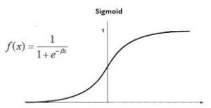
It is based on sigmoid function where output is probability and input can be from -infinity to +infinity.
Theory
Logistics regression is also known as generalized linear model.
As it is used as a classification technique to predict a qualitative response, Value of y ranges from 0 to 1 and can be represented by following equation:
p is probability of characteristic of interest.
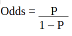
The odds ratio is defined as the probability of success in comparison to the probability of failure.
It is a key representation of logistic regression coefficients and can take values between 0 and infinity.
Odds ratio of 1 is when the probability of success is equal to the probability of failure.
Odds ratio of 2 is when the probability of success is twice the probability of failure.
Odds ratio of 0.5 is when the probability of failure is twice the probability of success.
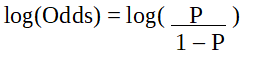
Since we are working with a binomial distribution(dependent variable), we need to choose a link function that is best suited for this distribution.
It is logit function.
In the equation above, the parenthesis is chosen to maximize the likelihood of observing the sample values rather than minimizing the sum of squared errors(like ordinary regression).
The logit is also known as a log of odds.
The logit function must be linearly related to the independent variables.
This is from equation A, where the left-hand side is a linear combination of x.
This is similar to the OLS assumption that y be linearly related to x.Variables b0, b1, b2 … etc are unknown and must be estimated on available training data.
In a logistic regression model, multiplying b1 by one unit changes the logit by b0.
The P changes due to a one-unit change will depend upon the value multiplied.
If b1 is positive then P will increase and if b1 is negative then P will decrease.
The Dataset
mtcars(motor trend car road test) comprises fuel consumption, performance and 10 aspects of automobile design for 32 automobiles.
It comes pre installed with dplyr package in R.
# Installing the package
install.packages("dplyr")
# Loading package
library(dplyr)
# Summary of dataset in package
summary(mtcars)
Performing Logistic regression on dataset
Logistic regression is implemented in R using glm() by training the model using features or variables in the dataset.
# Installing the package
install.packages("caTools")
# For Logistic regression
install.packages("ROCR")
# For ROC curve to evaluate model
# Loading package
library(caTools)
library(ROCR)
# Splitting dataset
split <- sample.split(mtcars, SplitRatio = 0.8)
split
train_reg <- subset(mtcars, split == "TRUE")
test_reg <- subset(mtcars, split == "FALSE")
# Training model
logistic_model <- glm(vs ~ wt + disp, data = train_reg,
family = "binomial")
logistic_model
# Summary
summary(logistic_model)
# Predict test data based on model
predict_reg <- predict(logistic_model, test_reg, type = "response")
predict_reg
# Changing probabilities
predict_reg <- ifelse(predict_reg > 0.5, 1, 0)
# Evaluating model accuracy
# using confusion matrix
table(test_reg$vs, predict_reg)
missing_classerr <- mean(predict_reg != test_reg$vs)
print(paste('Accuracy =', 1 - missing_classerr))
# ROC-AUC Curve
ROCPred <- prediction(predict_reg, test_reg$vs)
ROCPer <- performance(ROCPred, measure = "tpr", x.measure = "fpr")
auc <- performance(ROCPred, measure = "auc")
auc <- auc@y.values[[1]]
auc
# Plotting curve
plot(ROCPer)
plot(ROCPer, colorize = TRUE,
print.cutoffs.at = seq(0.1, by = 0.1),
main = "ROC CURVE")
abline(a = 0, b = 1)
auc <- round(auc, 4)
legend(.6, .4, auc, title = "AUC", cex = 1)wt influences dependent variables positively and one unit increase in wt increases the log of odds for vs =1 by 1.44.
disp influences dependent variables negatively and one unit increase in disp decreases the log of odds for vs =1 by 0.0344.
Null deviance is 31.755(fit dependent variable with intercept) and Residual deviance is 14.457(fit dependent variable with all independent variable).
AIC(Alkaline Information criteria) value is 20.457 i.e the lesser the better for the model.
Accuracy comes out to be 0.75 i.e 75%.Model is evaluated using the Confusion matrix, AUC(Area under the curve), and ROC(Receiver operating characteristics) curve.
In the confusion matrix, we should not always look for accuracy but also for sensitivity and specificity.
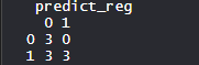
ROC and AUC curve is plotted.Output:Evaluating model accuracy using confusion matrix:
There are 0 Type 2 errors i.e Fail to reject it when it is false.
Also, there are 3 Type 1 errors i.e rejecting it when it is true.
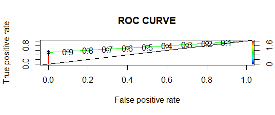
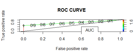
ROC curve:
In ROC curve, the more the area under the curve, the better the model.
ROC-AUC Curve:
AUC is 0.7333, so the more AUC is, the better the model performs.
naive-bayes-classifier

 Logistic regression is also known as Binomial logistics regression.
It is based on sigmoid function where output is probability and input can be from -infinity to +infinity.
Logistic regression is also known as Binomial logistics regression.
It is based on sigmoid function where output is probability and input can be from -infinity to +infinity.
 Since we are working with a binomial distribution(dependent variable), we need to choose a link function that is best suited for this distribution.
 It is logit function.
In the equation above, the parenthesis is chosen to maximize the likelihood of observing the sample values rather than minimizing the sum of squared errors(like ordinary regression).
The logit is also known as a log of odds.
The logit function must be linearly related to the independent variables.
This is from equation A, where the left-hand side is a linear combination of x.
This is similar to the OLS assumption that y be linearly related to x.Variables b0, b1, b2 … etc are unknown and must be estimated on available training data.
In a logistic regression model, multiplying b1 by one unit changes the logit by b0.
The P changes due to a one-unit change will depend upon the value multiplied.
If b1 is positive then P will increase and if b1 is negative then P will decrease.
It is logit function.
In the equation above, the parenthesis is chosen to maximize the likelihood of observing the sample values rather than minimizing the sum of squared errors(like ordinary regression).
The logit is also known as a log of odds.
The logit function must be linearly related to the independent variables.
This is from equation A, where the left-hand side is a linear combination of x.
This is similar to the OLS assumption that y be linearly related to x.Variables b0, b1, b2 … etc are unknown and must be estimated on available training data.
In a logistic regression model, multiplying b1 by one unit changes the logit by b0.
The P changes due to a one-unit change will depend upon the value multiplied.
If b1 is positive then P will increase and if b1 is negative then P will decrease.
 There are 0 Type 2 errors i.e Fail to reject it when it is false.
Also, there are 3 Type 1 errors i.e rejecting it when it is true.
ROC curve:
There are 0 Type 2 errors i.e Fail to reject it when it is false.
Also, there are 3 Type 1 errors i.e rejecting it when it is true.
ROC curve:
 In ROC curve, the more the area under the curve, the better the model.
ROC-AUC Curve:
In ROC curve, the more the area under the curve, the better the model.
ROC-AUC Curve:
 AUC is 0.7333, so the more AUC is, the better the model performs.
naive-bayes-classifier
AUC is 0.7333, so the more AUC is, the better the model performs.
naive-bayes-classifier